GGPlot2 is a fantastic library that allows you to build many complex graphs in R. However, it is a very powerful and complex tool that requires a lot of practise to master. Like anything, it has it’s own quirks.

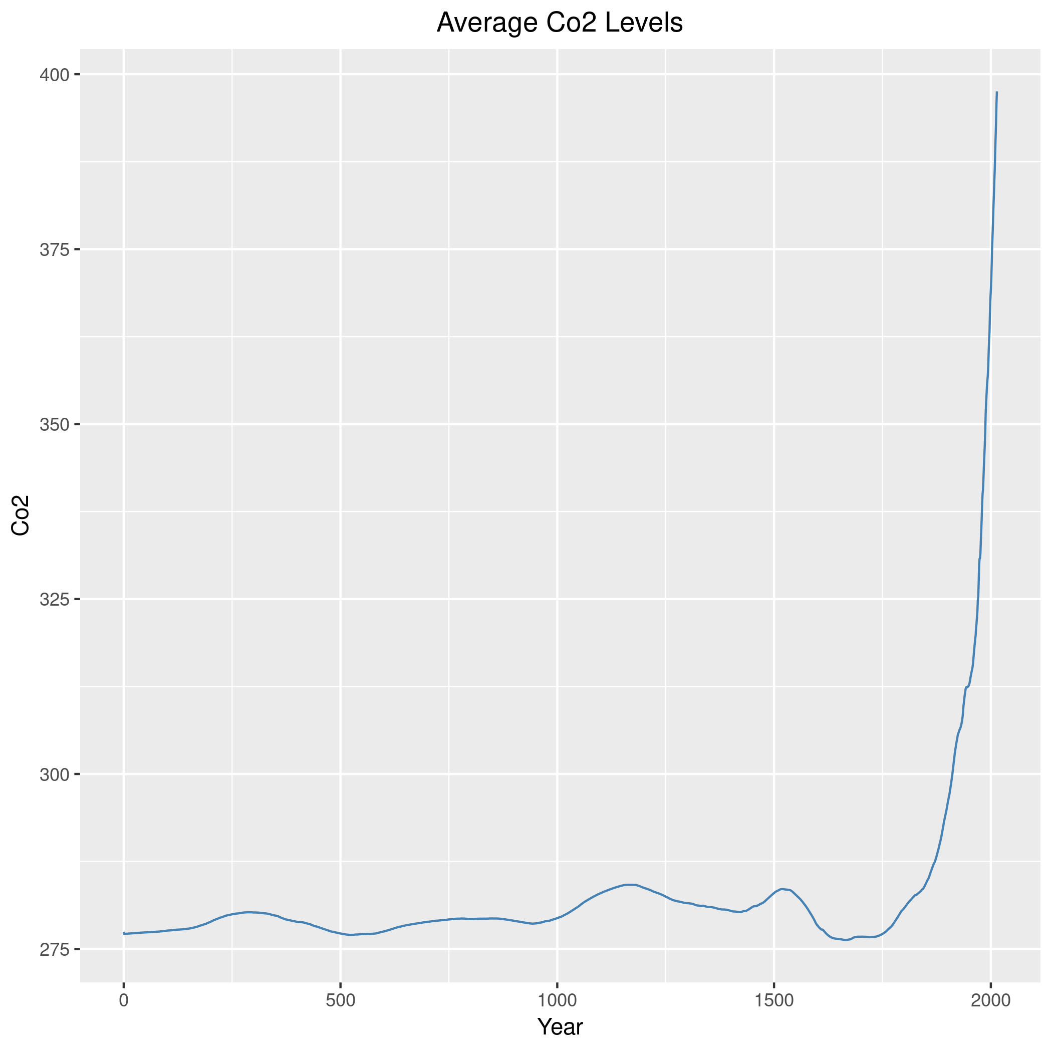
One that I’ll explore today, is that of the axis ticks, in our case, the X-Axis ticks, otherwise known as the labels of the graph. I’ve used data from Co2 Datasets with measurments of the mean Co2 levels from 0 AD to 2014.

When plotted with GGPlot, the library does everything for us and gives a nice plot, whilst simplyifying the X-Axis.

ggplot( data = lDataMelt, aes( year, y = value, group = variable ) ) +
  geom_line( color = "steelblue" ) +
  ggtitle("Average Co2 Levels") +
  ylab( "Co2" ) +
  xlab( "Year" ) +
  theme( plot.title = element_text( hjust = 0.5 ) )

However, often we may want to display more (or less) detail on the axis. To do this we can use the scale_x_continuous function, setting the breaks to be the sequence (every label) from the dataframe.

scale_x_continuous( breaks = seq( min( lDataMelt$year ), max( lDataMelt$year ) ) )

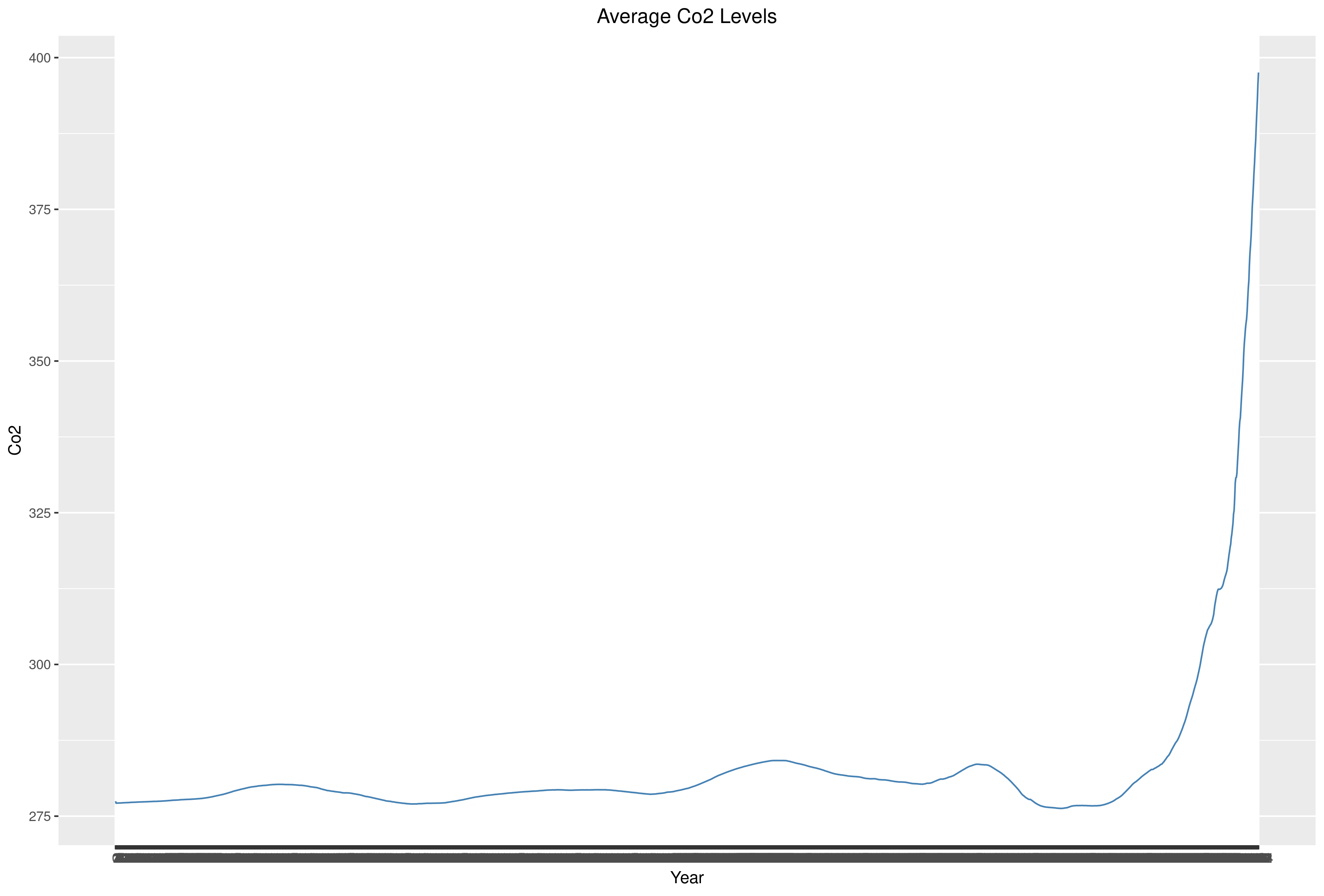
Unfortunately, that’s really ruined things, however, one trick to hide the number of ticks displayed is this handy little function I’ve written.

createLabels <- function( aTable, show )
{
  lLabels <- vector( length = dim( aTable )[1] )
  for(i in 1:( dim(aTable)[1] ) )
  {
    if( i %% show == 0)
      lLabels[i] <- rownames( aTable )[i]
    else
      lLabels[i] <- ""
  }
  lLabels
}

The createLabels function will only show the number of labels given by the show parameter. EG is show = 3, then it will show only every 3rd tick. We can then simply add it to *scale_x_continuous with the labels parameter. In our case, we’ll use 100, to show every 100th label. We’ve also rotated the ticks slightly.

scale_x_continuous( breaks = seq( min( lDataMelt$year ), max( lDataMelt$year ) ), labels = createLabels( lDataMelt, 100 ) )

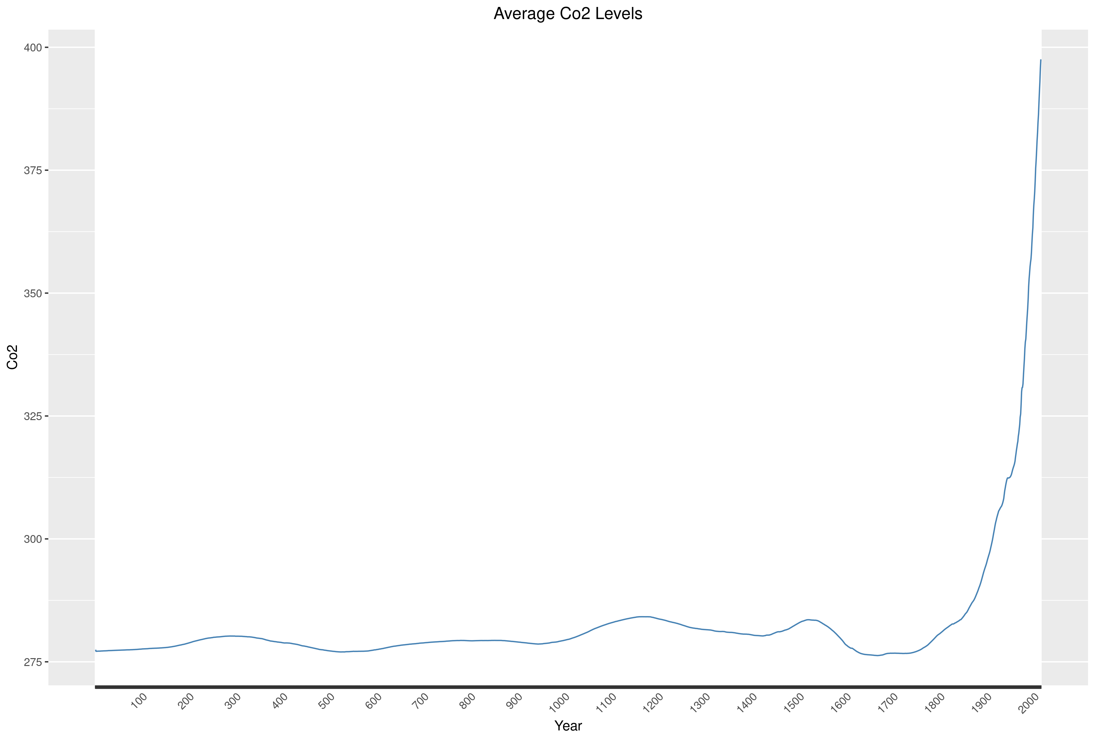
There you have it, much tidier now.

The source code can be found here.